💔 Decorrelation + Deep learning = Generalization
The most pervasive challenge in deep learning is Overfitting . This occurs when the dataset is small, and extensive training leads to a model that excels on training datasets but fails to generalize to validation datasets or real-world scenarios. To address this issue, various strategies have been developed. Historically, in statistics, regularization methods like Ridge and LASSO were employed, while deep learning has adopted approaches such as regularizing weights or applying different techniques to neural networks. These techniques encompass a range of methods.
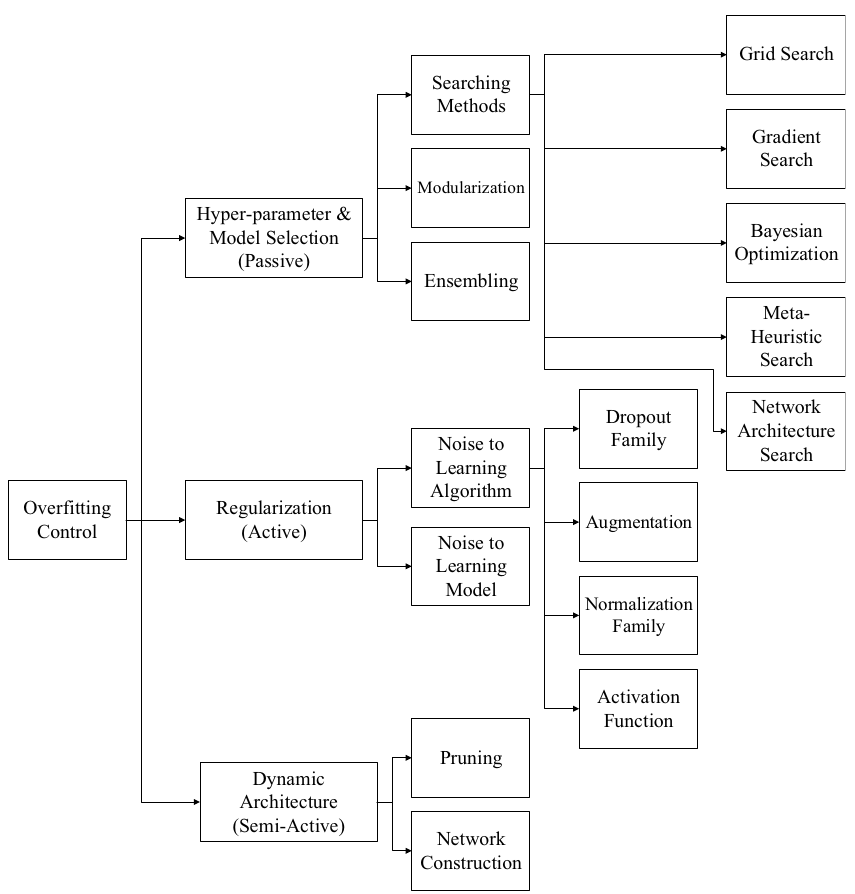
Bejani, M.M., Ghatee, M. A systematic review on overfitting control in shallow and deep neural networks. Artif Intell Rev 54, 6391-6438 (2021)
Among these, Dropout is perhaps the most well-known, which involves omitting certain neurons in a neural network to prevent their co-adaptation. Practically, this has proven to be an exceedingly effective measure to mitigate overfitting, becoming a standard inclusion in neural network architectures. However, dropout is not universally applicable: with limited training data or few neurons, the random removal of neurons might impede the network’s capacity to model complex relationships. Additionally, despite its practicality, dropout’s straightforward architecture and the principle may seem less theoretically satisfying. In this context, I wish to present an intriguing paper that offers both theoretical enrichment and practical effectiveness.
1. Why do we need decorrelation?
1.1. Covariance & Correlation
The paper under review, Reducing Overfitting in Deep Networks by Decorrelating Representations from 2015, introduces a method termed Decorrelation . The authors demonstrate how this technique can bolster the performance of Dropout in reducing overfitting. Despite its potential, Decorrelation did not surge in popularity, likely due to its novelty and relative complexity. Nevertheless, it remains a valuable and consistently cited work in the field.
To grasp the concept of decorrelation, we must first understand what correlation entails. Correlation denotes the relationship between two sets of data, with covariance being a common measure of this relationship. Covariance is defined as the linear association between two random variables, expressed by the formula:
$$ \text{Cov}(X,\,Y) \equiv \mathbb{E}\left[(X-\mathbb{E}[X])(Y-\mathbb{E}[Y])\right] $$
It is generally understood that a positive covariance indicates a direct proportional relationship between variables, a negative value suggests an inverse relationship, and a value near zero implies no apparent relationship. A more precise metric for this relationship is the Pearson correlation coefficient, defined as:
$$ \text{Corr}(X,\,Y) \equiv \frac{\text{Cov}(X,\,Y)}{\sqrt{\text{Var}(X) \text{Var}(Y)}} $$
This coefficient is constrained within a range from -1 to 1. A value closer to 1 indicates a strong direct relationship, closer to -1 indicates a strong inverse relationship, and a value near 0 suggests no correlation. Consider the following data as an illustration.
# Python
import numpy as np

x = np.array([1,2,3,4])
y = np.array([5,6,7,8])
For these two variables, the covariance can be calculated using the following function in Python:
# Python
def cov(x, y):
    N = len(x)
    m_x = x.mean()
    m_y = y.mean()
    return np.dot((x - m_x), (y - m_y)) / (N-1)
Using this function to compute the covariance for x and y above yields a value of 1.6666666666666667. This indicates a positive correlation, but interpreting this raw number can be challenging. To facilitate a clearer interpretation, we employ the Pearson correlation coefficient, as previously mentioned, defined in Python as:
# Python
def pearson_corr(x, y):
    # ddof=1 for sample variance
    return cov(x, y) / np.sqrt(x.var(ddof=1) * y.var(ddof=1))
Applying this to the given data reveals a Pearson correlation coefficient of exactly 1, signifying that the two variables have a perfect linear relationship.
When dealing with multiple features, it is possible to construct a matrix that represents the covariance among them all at once. This is known as the covariance matrix, and is denoted as follows:
$$ C_{ij} = \text{Cov}(x_i,\,x_j) $$
Therefore, the covariance matrix is a square matrix with dimensions equal to the number of features, representing the covariance between each pair of features.
1.2. Overfitting & Decorrelation
The discussion of correlation in the realm of deep learning arises from the issue that significant correlation among variables, or features, can be detrimental to a model’s performance. Deep neural networks refine their learning by adjusting weights assigned to each feature; however, when two features yield identical information (high correlation), it creates redundancy. This redundancy can cause a form of degeneracy where altering the weights of either feature doesn’t uniquely contribute to the learning process, which in turn can impede accurate learning and introduce bias into the neural network. The aforementioned paper posits that this redundancy is a contributing factor to overfitting.
In fact, the study demonstrates that by defining the extent of overfitting as the discrepancy between training and validation accuracy and quantifying the level of decorrelation with a metric termed DeCov, a notable pattern emerges:

Correlation between Overfitting and Covariance
The graph above illustrates that with an increase in the number of training samples, the degree of overfitting diminishes, concurrently with a decrease in Cross-Covariance. This correlation suggests that by reducing covariance, or in other words, promoting decorrelation, one can potentially reduce the tendency of a model to overfit.
2. How to decorrelate?
Within the paper, the authors propose that to combat overfitting, one should aim to decorrelate the activation outputs of the hidden layers. This approach is grounded in the logic that these activations are the actual values being multiplied by subsequent weights in the network. Let’s consider the activation values of one hidden layer as $h^n \in \mathbb{R}^d$, where $n$ is the batch index. We can then define the covariance matrix of these activations as:
$$ C_{ij} = \frac{1}{N} \sum_n (h_i^n - \mu_i)(h_j^n - \mu_j) $$
By reducing the covariance of these activation values, we aim to achieve our objective of decorrelation. However, to integrate this concept into our Loss function, which requires a scalar value, the covariance matrix must be represented in a scalar form. The paper introduces the following Loss function for this purpose:
$$ \mathcal{L}_{\text{DeCov}} = \frac{1}{2}(\lVert C \rVert_F^2 - \lVert\text{diag}(C) \rVert_2^2) $$
Here, $\lVert \cdot \rVert_F$ denotes the Frobenius norm of the matrix, and $\lVert \cdot \rVert_2$ denotes the $l^2$ norm. The subtraction of the diagonal components is deliberate since these represent the variance of individual features, which does not contribute to inter-feature correlation. By incorporating this DeCov Loss function into the overall loss, much like a regularization term, we can enforce decorrelation in the learning process.
Implementing this decorrelation strategy in practical deep learning applications may initially appear daunting, given the complexity of gradient calculations for the covariance matrix and its norms. However, PyTorch simplifies the process considerably with its built-in automatic differentiation capabilities, which can handle gradients for the covariance matrix and norms with ease. Consequently, this DeCov loss function can be integrated into your model with just a few lines of Python code:
# Python
import torch

def decov(h):
    C = torch.cov(h)
    C_diag = torch.diag(C, 0)
    return 0.5 * (torch.norm(C, 'fro')**2 - torch.norm(C_diag, 2)**2)
By defining a function decov, we calculate the covariance matrix C of the activations h. The function then computes the DeCov loss by taking the Frobenius norm of the entire covariance matrix, squaring it, and subtracting the squared $l^2$ norm of the diagonal elements, which represent the variance of each feature. This DeCov loss can then be added to the primary loss function, thereby enabling the model to learn decorrelated features effectively.
3. Apply to Regression
In the original study, the authors applied their decorrelation technique to various sets of image data. However, to more clearly demonstrate its effectiveness, we’ll apply it to a simple regression problem. Below is the dataset that will be used to train the neural network:
![Nonlinear data [Note: Peroxide_Gallery]](/posts/images/005_04_data.png)
Nonlinear data [Note: Peroxide_Gallery]
To illustrate the impact of the DeCov loss function, we will compare the performance of a standard neural network to one that implements the DeCov function. The architecture of the neural network utilizing DeCov is detailed below.
import pytorch_lightning as pl
from torch import nn
import torch.nn.functional as F
# ...

class DeCovMLP(pl.LightningModule):
    def __init__(self, hparams=None):
        # ...

        self.fc_init = nn.Sequential(
            nn.Linear(1, self.hidden_nodes),
            nn.ReLU(inplace=True)
        )

        self.fc_mid = nn.Sequential(
            nn.Linear(self.hidden_nodes, self.hidden_nodes),
            nn.ReLU(inplace=True),
            nn.Linear(self.hidden_nodes, self.hidden_nodes),
            nn.ReLU(inplace=True),
            nn.Linear(self.hidden_nodes, self.hidden_nodes),
            nn.ReLU(inplace=True),
        )

        self.fc_final = nn.Linear(self.hidden_nodes, 1)

        # ...

    def forward(self, x):
        x = self.fc_init(x)
        x = self.fc_mid(x)
        return self.fc_final(x)

    def training_step(self, batch, batch_idx):
        x, y = batch

        h0 = self.fc_init(x)
        loss_0 = decov(h0)

        h1 = self.fc_mid(h0)
        loss_1 = decov(h1)

        y_hat = self.fc_final(h1)
        loss = F.mse_loss(y,y_hat) + loss_0 + loss_1

        return loss

    # ...
Upon closer examination, we observe that loss_0 is defined as the loss after the initial layer fc_init, and loss_1 as the loss after the subsequent three layers fc_mid. These losses are then integrated into the mean squared error (MSE) loss as regularization terms. Before delving into the outcomes, it’s insightful to examine the training dynamics of SimpleMLP and DeCovMLP.
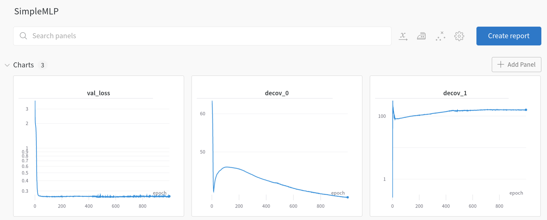
SimpleMLP losses (wandb.ai)
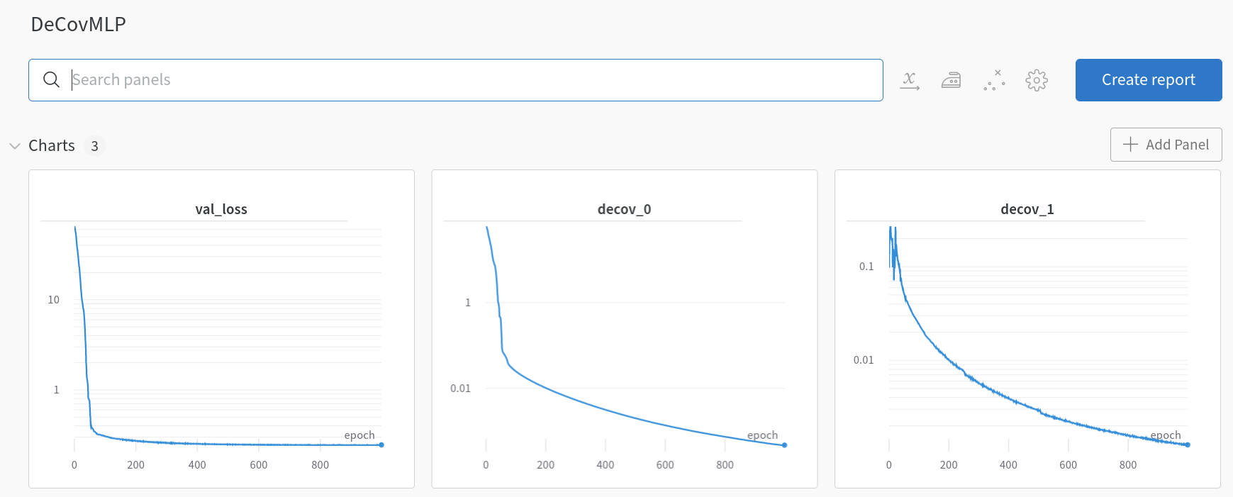
DeCovMLP losses (wandb.ai)
In the SimpleMLP model, decov_1 initially increases during training iterations and then plateaus, indicating no further decrease. Contrastingly, within the DeCovMLP model, decov_1 consistently decreases, aligning with the paper’s hypothesis: as overfitting intensifies, so does the correlation between features. Now, let’s consider the results.
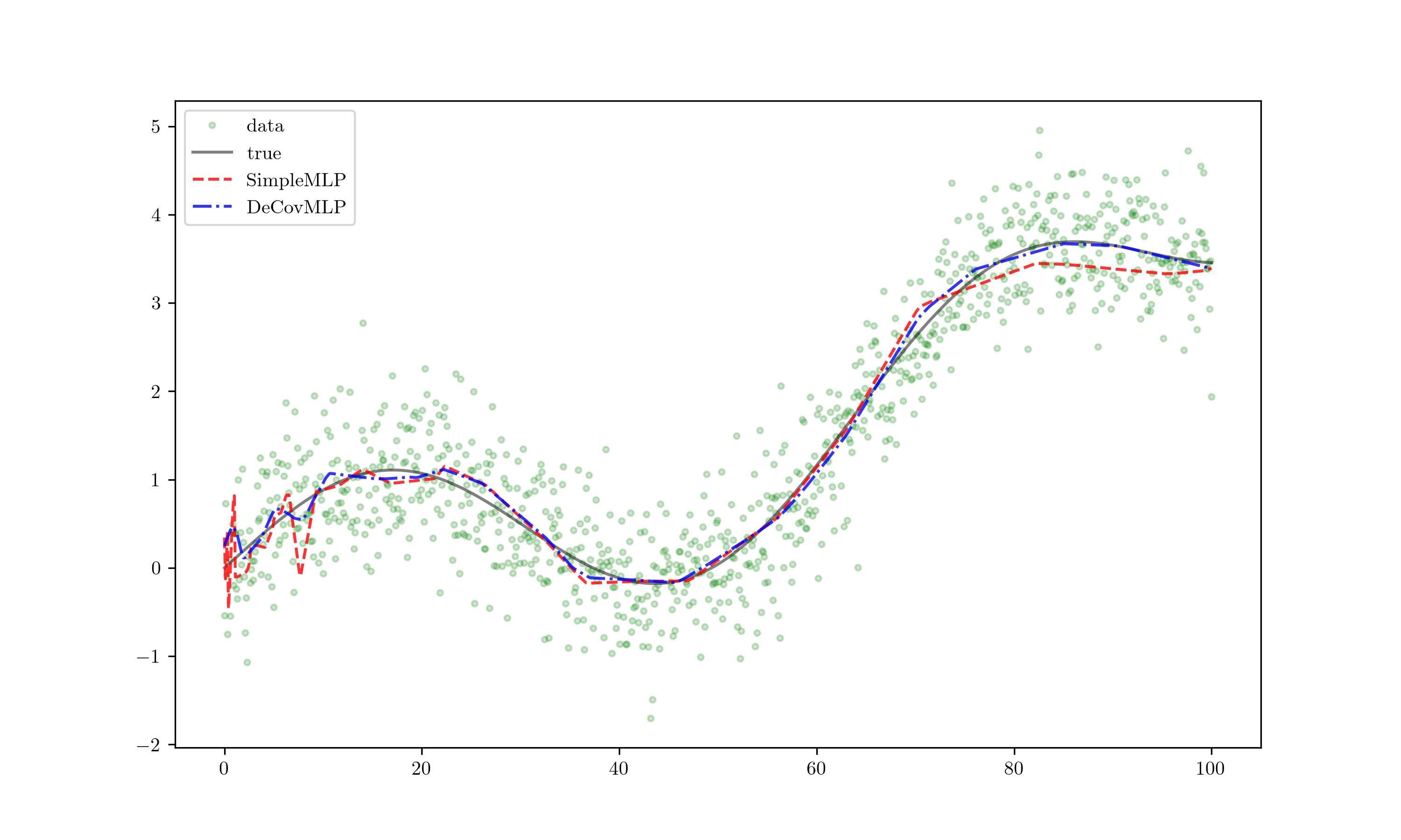
Results!
The red line represents the SimpleMLP outcome, while the blue line depicts DeCovMLP. Noticeably, the red line exhibits overfitting with erratic fluctuations, whereas the blue line maintains closer alignment with the true data and exhibits less jitter. This demonstrates a remarkable improvement, and further extrapolation yields even more compelling insights.
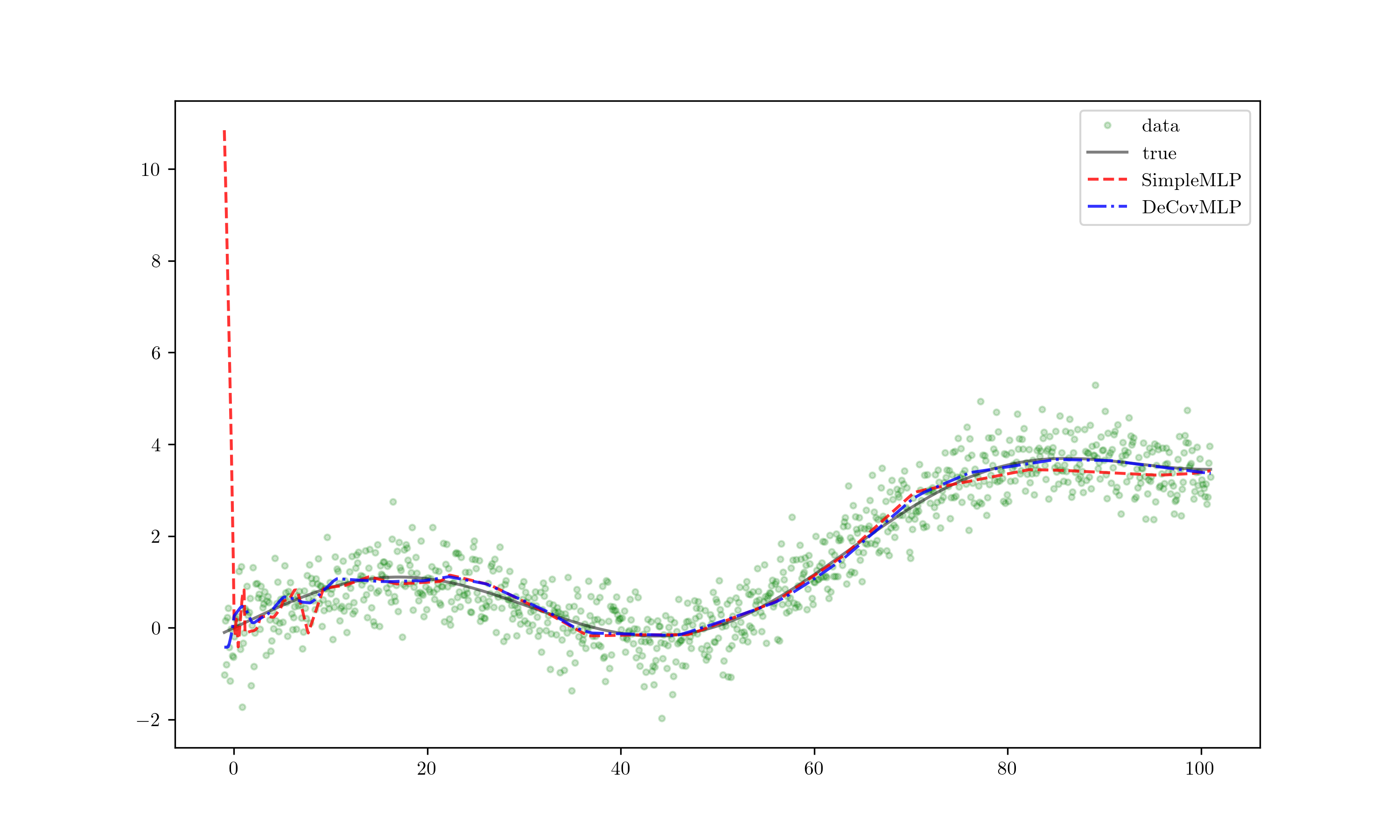
Extrapolate!
When extrapolated, the red line — indicative of overfitting — diverges significantly from the expected trend even with minor deviations, leading to inaccurate predictions. Meanwhile, the blue line remains stable, displaying minimal deviation. This clearly demonstrates the superior generalization capability of the DeCovMLP.
4. Further more..
The paper, “Reducing Overfitting in Deep Networks by Decorrelating Representations,” was published in 2015—a notable period ago, especially when considered within the fast-paced advancements of the field up to 2022. Since its publication, there has been a continuous outpouring of research on decorrelation techniques, with studies like Decorrelated Batch Normalization emerging more recently. Decorrelation, having been extensively explored in the field of statistics, offers a robust theoretical foundation that can render the results of neural networks more intuitive and analytically solid for researchers and practitioners alike.
For those interested in delving deeper, the regression code discussed earlier can be accessed at the provided link.